suppressWarnings({

options(digits = 3, scipen = 99999, warn = -1)
  remove(list = ls())
  graphics.off()

suppressPackageStartupMessages(library(tidyverse))
suppressPackageStartupMessages(library(ggthemes))
suppressPackageStartupMessages(library(crayon))
suppressPackageStartupMessages(library(qreport))
suppressPackageStartupMessages(require(data.table))
suppressPackageStartupMessages(library(binom))
suppressPackageStartupMessages(library(bbdetection))
suppressPackageStartupMessages(library(data.table))
suppressPackageStartupMessages(library(boot))
suppressPackageStartupMessages(library(mixR))
suppressPackageStartupMessages(library(ggjoy))
suppressPackageStartupMessages(library(hrbrthemes))
suppressPackageStartupMessages(library(ggridges))

})Confidence Intervals via Bootstrap for the Mean of a Population with Many Zero Values
Data underlying practically all Medicaid Audits entail a population that contains a disproportionately large amount of zeros. A zero is booked when a particular filing is in compliance.
This artifact is known as a zero-inflated population (“ZIP”) and refers to the observed spike at zero value in a frequency distribution.
The identified overpayments are, in turn, drawn from an unknown distribution. In fact, we model the estimation of a provider’s liability as a mixed distribution reflecting dual data-generating-processes.
This characterization of the DGP can be seen in the graph below for the resulting mixture as well as the two constituent distributions: a Bernoulli distribution with a success (“1”) probability of 0.10 and a Normal (5,1) distribution characterizing the overpayments. These distribution parameters are plausible values in medicaid audits.
suppressWarnings({
b1<-data.frame(DGP= "Bernoulli (0.10)", Values = rbinom(size = 1, 500, prob= .10))
          b2<-data.frame(DGP= "Normal(5,1)", Values = rnorm(500, 5, 1))
          b3<-data.frame(DGP= "Mixture",
                         Values = rbinom(size = 1, 500, prob= .10)*
                                  rnorm(500, 5, 1))
          df<-rbind(b1,b2,b3)

          ggplot(df, aes(x=Values, y=DGP, fill = as.factor(DGP)))+
            geom_joy(scale = 2, alpha=0.25) +
            scale_y_discrete(expand=c(0.01, 0)) +
            scale_x_continuous(expand=c(0.01, 0)) +
            theme_joy() +
            theme_ipsum_tw() +
            theme(legend.position = "NULL")
})
Picking joint bandwidth of 0.252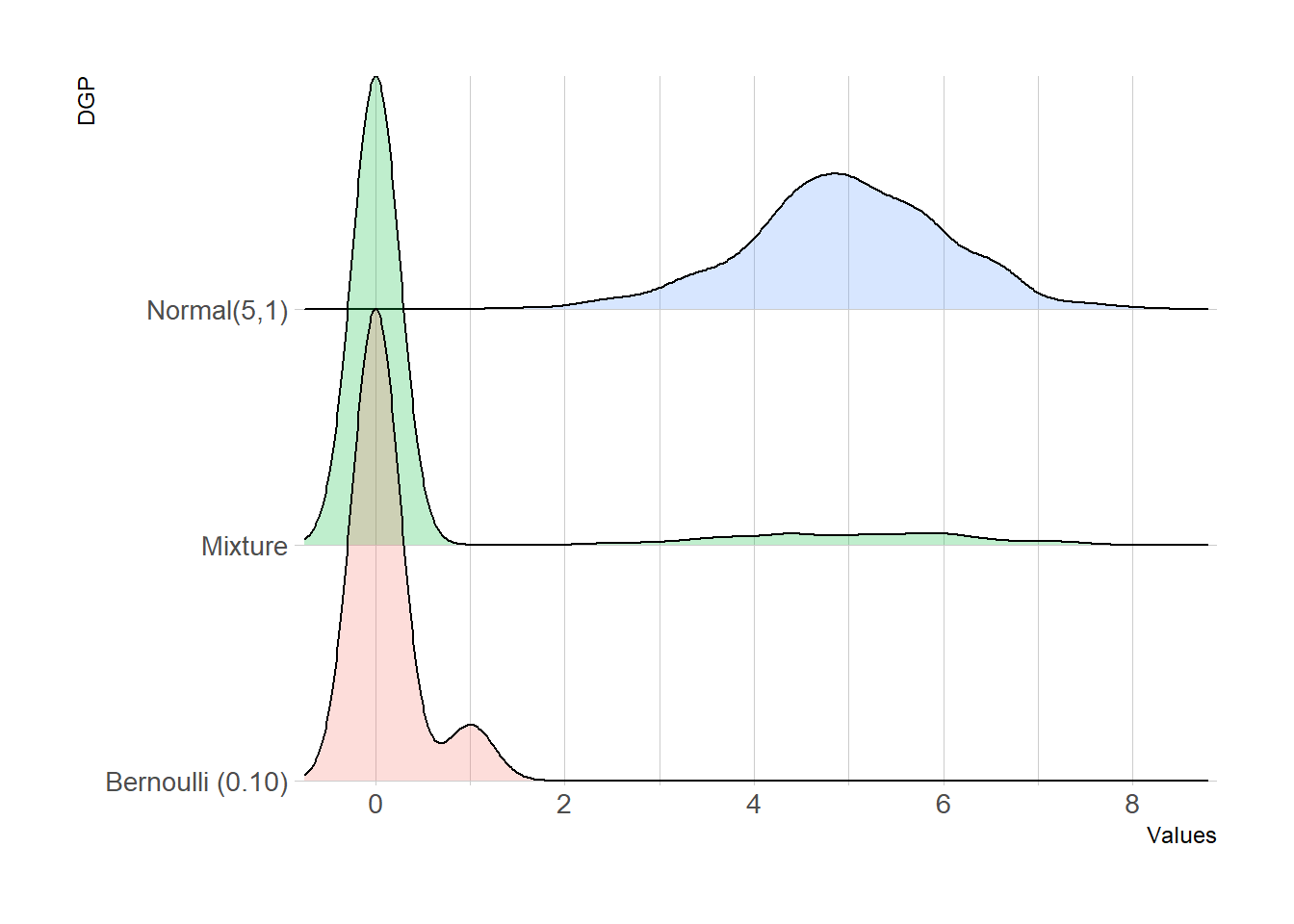
A mixture containing zero-inflated data results in a zero-inflated, highly skewed distribution. This non-conformity with normality assumptions weakens the theoretical statistical rationale underscoring the confidence intervals built into audit procedures.
“Specifically, a sample taken from this type of population usually consists of a very large number of zero values, plus a small number of non-zero values that follow some continuous distribution. In this situation, the traditional confidence interval constructed for the population mean is known to be unreliable.” (Kvanli, Shen, & Deng, 1998)1
See also,
Chen, Jiahua, Shun-Yi Chen, and J.N.K. Rao, “Empirical Likelihood Confidence Intervals for the Mean of a Population Containing Many Zero Values,” The Canadian Journal of Statistics, Vol. 31, No.1, (2003), pp: 53-68.
Paneru, Khyam, R. Hoah Padgett, and Hangfen Chen, “Estimation of Zero-Inflated Population Mean: a Bootstrapping Approach,” Journal of Modern Applied Statistical Methods, Vol 17, No. 1 (May 2018), pp: 2-14.
Medicaid auditors rely on classical 95% nominal confidence levels based on the Central Limit Theorem (CLT) for the construction of confidence intervals for the mean of audit results. These mean values are key in establishing a provider’s alleged liability.
We show here how the presence of ZIPs vitiates reliance on CLT-based measures. Specifically, we show two things in this tutorial: (i) that the coverage percentage is vitiated in the presence of ZIPS for two instances of non-zero distributions, and (ii) that bootstrapping means provides dependable confidence intervals.
Medicaid Audits
The Medicaid Fraud Control Units (MFCUs) is an enforcement unit typically housed within a State Attorney General’s office. MFCUs conduct audits of service providers to determine whether they have inappropriately billed a state Medicaid program.
MFCU auditors comb through the sampled claims and identify, or flag, claims that appear to have been paid in excess (or claims paid less than the amounts claimed). These flagged claims are coded as non-zeroes in the sample dataset used in the empirical analysis. The claims that are properly booked and not flagged are coded as zeroes. Because only a handful of the randomly-sampled and audited claims are typically disputed the result is a zero-inflated dataset.
It is common practice to assume an approximately normal distribution to construct confidence intervals marking the confines of a provider’s liability. In fact, the process in which confidence intervals derived from assuming normality are baked-in into Rat-Stats - the MFCU’s in-house statistical package. Rat-Stats is an open-source platform available for public use. 2
Modeling
In medicare audits, a small sample of about 100-400 claims are often obtained for examination. Most of these claims will be sound, but a small portion of claims may be non-zero.
Simulation Procedure
To carry out the simulation experiments, we assume that the error rate p varies from .05 to .30 in increments of .05 the mean of the error distribution was also specified in each experiment, and the sample size was set from n = 100 to 400 varying in increments of 100.
For each of the nonzero value distributions generated, we compute the coverage percentage for the (1) the traditional method (classical method based on CLT), (2) the normal algorithm, and the exponential algorithm. The coverage percentage is measures as the percentage of times (out of 1000) that the population mean is inside the confidence limits.
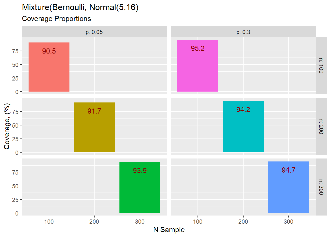
We give a summary finding for our simulation study and present only tables with sample sizes of n = 100, 200, and 300, and p value (the proportion of non-zeroes) of p = 0.05 and p = 0.30.
The first result is for the normal distribution with a mean of 5 and a standard deviation of 16.
create_y  <- function(n, p,  mu1, sigma1) {
              k <- stats::rbinom(n,size = 1, prob = p)
              y = k*rnorm(n, mu1, sigma1)
              #y = k*rexp(n, rate = 1/mu1)
              #y = k*1
            }
            #
            ssum = numeric(1000)
            n = c(100,200, 300)
            #n = 200
            pee = c(0.05, 0.10, 0.15, 0.20, 0.25,0.3)
            mydata = expand.grid(n = n,p = pee)
            setDT(mydata)

            #i = 1
            for( i in 1:nrow(mydata)){
              for (k in 1:1000){
                w = mydata[i,]
                p = w$p
                n = w$n
                mu1 = 5
                sigma1 = 16
                y = create_y(n,p, mu1 = mu1, sigma1 = sigma1)
                pop_mean = p*mu1
                ttmu = t.test(mu = pop_mean, x = y )
                ssum[k] = between(pop_mean,ttmu$conf.int[1], ttmu$conf.int[2] )
                mean_ssum = mean(ssum)

              }

              mydata[i, "Coverage,%" := mean_ssum*100]
              mydata[i,Lower_Bound := ttmu$conf.int[1]]
              #i = i +1
            }
            setDF(mydata)
            colnames(mydata)[3] = "Coverage"

    ggplot(mydata
        #%>% filter(p == 0.05)
                   %>% filter(p %in% c(0.05, 0.30))
                   ,
                   aes(x = as.factor(n)
                                          ,y = Coverage,
                       fill = as.factor(Coverage)
                                                                  )) +
              geom_bar(stat = "identity",
                       position = "dodge") +
              geom_text(aes(label = Coverage ), vjust = 2, colour = "darkred")+
              #coord_flip()+
              facet_grid(
                n~p,
                         labeller = label_both) +
              theme(legend.position = "NULL") +
              labs(
                x= "N Sample",
                y = "Coverage, (%)",
                title = "Mixture(Bernoulli, Normal(5,16)",
                subtitle= "Coverage Proportions"
              )
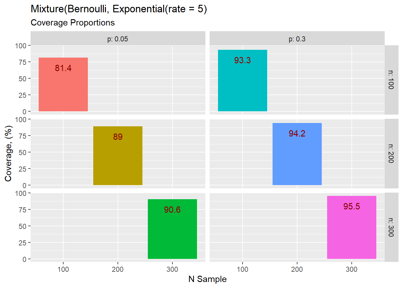
The exponential with rate of 5.
Many resampling methods have been proposed for gauging the accuracy of the confidence intervals. Resampling methods have the ability to eliminate the effect of skewness.
suppressWarnings({

        (  pee = seq(from = 0.05, to = 0.30, by = 0.05)   )
        (  en = seq(from = 100, to = 400, by = 100)  )
        mydf = expand.grid(n = en, p = pee)
        setDT(mydf)
        head(mydf)


        create_y  <- function(n, prob = p,  mu1, sigma1) {
          k <- rbinom(size = 1, n, prob)
          y = k*rnorm(n, mu1, sigma1)
          #y = k*rexp(n, rate = 1/6)
          #y = k*1
        }


        mixedy  <- function(data,indices) {
          d = data[indices,]
          mean(d)
        }


        for (i in 1:nrow(mydf)){
          w = mydf[i,]
          n = w$n
          p = w$p
          mu1 = 5
          sigma1  = 16
          y_created = create_y(n,p, mu1 = mu1, sigma1 = sigma1)
          meanval = mean(y_created)

          data = y_created %>% as.data.frame()
          boot_out <- boot(
            data,
            R = 1000,
            statistic = mixedy
          )
          ci = boot.ci(boot_out, type = "all")
          set(mydf,i, "True value", meanval)
          mydf[i,Normal_LL := ci$normal[1,2]]
          mydf[i,Normal_UL := ci$normal[1,3]]
          #mydf[i,Basic_CI_L := ci$basic[1,4]]
          #mydf[i,Basic_CI_R := ci$basic[1,5]]
          mydf[i,BCA_LL := ci$bca[1,4]]
          mydf[i,BCA_UL := ci$bca[1,5]]
        }

        mydf %>% filter(p %in% c(0.05, 0.30))
})
n p True value Normal_LL Normal_UL BCA_LL BCA_UL
1: 100 0.05 -0.0668 -0.3539 0.216 -0.8276 0.060
2: 200 0.05 0.2530 -0.1604 0.684 -0.1087 0.751
3: 300 0.05 0.0805 -0.3884 0.522 -0.3543 0.576
4: 400 0.05 0.2650 -0.0728 0.592 -0.0147 0.699
5: 100 0.30 1.7364 -0.3571 3.802 -0.1156 4.206
6: 200 0.30 2.0964 0.7307 3.419 0.8222 3.470
7: 300 0.30 3.1208 1.9836 4.257 2.0090 4.294
8: 400 0.30 1.9386 1.1814 2.740 1.2842 2.820Concluding Comment
We have shown the limitations of relying on traditional Central Limit Theorem-based confidence intervals to establish provider liability in medicare audits.
We also demonstrated how the use the bootstrap method to compute confidence intervals of a zero-inflated population.
Footnotes
Kvanli, Alan H., Yaung Kaung Shen, & Lih Yuan Deng., “Construction of Confidence Intervals for the Mean of a Population Containing Many Zero Values,” Journal of Business and Economic Statistics, Vol. 16, No. 3 (July, 1998).↩︎
Source: https://oig.hhs.gov/compliance/rat-stats/ (viewed: January 27, 2023)↩︎