options(digits = 3, scipen = 9999)
remove(list = ls())
graphics.off()

suppressWarnings({
suppressPackageStartupMessages({
library(janitor)
library(tidyverse)
library(forcats)
library(explore)
library(finalfit)
library(lubridate)
library(readxl)
library(forecast)
library(TSstudio)
library(tsbox)
library(car)
})})When Data Drifts
“… overreliance on any descriptive statistic can lead to misleading conclusions, or cause undesirable behavior.”
Charles Wheelan, Naked Statistics
The formal process of exchanging information in preparation for trial, known as discovery, compels parties to produce financial documents, business records, and other data that may have a bearing on the case at hand. Once data are disclosed it is not common practice for financial or economic experts to scrutinize the soundness of the data per se.
But the data may be have changed - either deliberately or unintentionally. So it may be productive to run a few tests before starting any analysis. I started on this theme and a survey of available tools and tests in an earlier tutorial. In this tutorial we will be concerned with what is known as data drift - a common occurrence in practice. Here I will discuss an actual instance of a data shift in a fraud case and then provide a more general example. Here we limit the analysis to the shift in one account over two periods, - and pick up a shift in the entire covariance set in a later tutorial.
Setup
There is an excellent example of this data artifact in Mark Nigrini’s excellent book: Forensic Analytics (2nd Edition, 2020), The chapter is titled, Comparing Current and Prior Period Data. Data used in the chapter are the purchasing card data for the District of Columbia which can be downloaded via the DC government’s open-data page. Nigirini’s objective is to determine whether descriptive statistics point to a difference in the data between 2011 and 2012. The period was chosen because high level testing revealed two anomalies in 2012 (the anomaly tests are not discussed in the chapter).
The ultimate objective of Nigrini’s approach is to call attention to the event presumably for further inquiry.
suppressWarnings({
mydata <- read_excel("PCard_Data2009-2014.xlsx")

})

mydata$...7 = NULL
I isolate the two years: 2011 and 2012 - following Nigrini.
mydata1112 = mydata |> dplyr::mutate(month = format(Date, "%m"), year = format(Date, "%y"))|>
            group_by(year) |>
          filter(year == "11" | year == "12")

my11 = mydata1112 |> filter(year == "11")
my12 = mydata1112 |> filter(year == "12")
The focus is on the transaction amounts. The following graph shows the distributions.
mydata1112 |> explore(Amount, target = year, split = TRUE)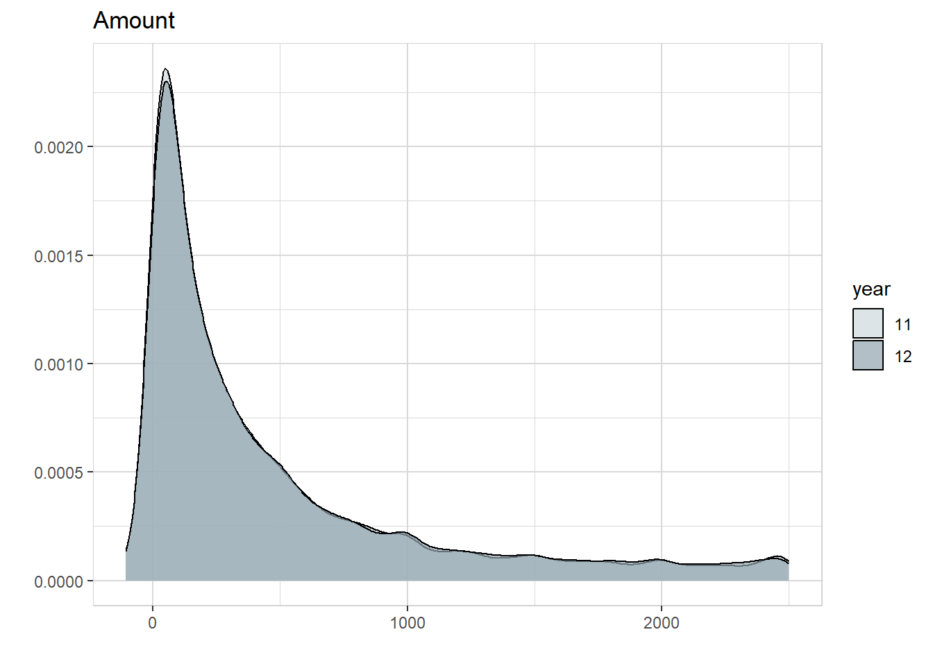
and here is a different perspective via the empirical cumulative distribution functions:
mya = ecdf(my11$Amount)
myb = ecdf(my12$Amount)
plot(myb, verticals = TRUE, do.points = FALSE, col = "darkblue", lwd = 2, main = "Amount, ($)")
plot(mya, add = TRUE, verticals = TRUE, do.points = FALSE, col = "darkred", lwd = 2)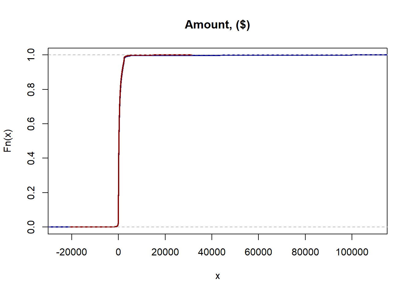
Truth to tell one can hardly notice anything visually.
Nigrini sets forth Year-to-Year changes across any number of summary statistics; and tests whether the changes are statistically significant.
A notable change in means for example.
t.test(Amount ~ year, data = mydata1112)
    Welch Two Sample t-test

data:  Amount by year
t = -9, df = 35557, p-value <0.0000000000000002
alternative hypothesis: true difference in means between group 11 and group 12 is not equal to 0
95 percent confidence interval:
 -227 -146
sample estimates:
mean in group 11 mean in group 12
             506              692
But more to the point, what I like in Nigrini’s approach is that he pushes beyond the changes in the mean and carefully examines changes in the variance, the nature of the distribution itself. He probes for changes in the quartiles, changes in variance, changes in the coefficient of variation, changes in the interquartile range, changes in the maximum.
This is thinking clearly; the simple test of means can beguile us into failing to recognize that the distribution of the account itself my vary year-to-year. See the graph below.
mydata1112 |>
    ggplot(aes(x = as.factor(year), y = Amount, col = as.factor(year))) +
    geom_boxplot()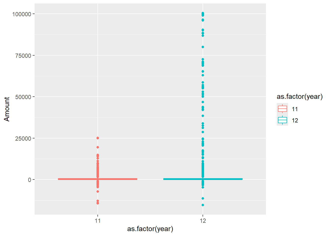
This is, for all intents and purposes, checking for data drift. The boxplots clearly show that the 2012 transaction was more variable than that of the previous year. We test whether the seeming increase in the number of large transactions is significant. Here are two of the battery of tests run by Nigrini.
var.test(Amount ~ year, data = mydata1112)
    F test to compare two variances

data:  Amount by year
F = 0.05, num df = 34319, denom df = 32462, p-value <0.0000000000000002
alternative hypothesis: true ratio of variances is not equal to 1
95 percent confidence interval:
 0.0494 0.0515
sample estimates:
ratio of variances
            0.0504
This test of variance can be done by hand - first obtaining the
A12 = mydata1112 |> filter(year == "12") |>
      dplyr::select(Amount)
Adding missing grouping variables: `year`A11 = mydata1112 |> filter(year == "11") |>
dplyr::select(Amount)Adding missing grouping variables: `year`suppressWarnings(
( myvar = var(A12$Amount)/var(A11$Amount))
)[1] 19.8and the p-value is the area of the density curve of the F distribution.
myp = 1 - pf(myvar, 34319,32462)Confirming the statistical significance.
The Levene test adds redundancy; it is used to determine whether the variances are equal.
suppressWarnings(
car::leveneTest(Amount ~ year, data = mydata1112)
)
Levene's Test for Homogeneity of Variance (center = median)
Df F value Pr(>F)
group 1 79.5 <0.0000000000000002 ***
66781
---
Signif. codes: 0 '***' 0.001 '**' 0.01 '*' 0.05 '.' 0.1 ' ' 1I personally prefer the Kologorov Smirnoff test - which surprisingly is not in Nigrini’s battery of tests.
suppressWarnings(
        ks.test(my11$Amount, my12$Amount)
                )
    Asymptotic two-sample Kolmogorov-Smirnov test

data:  my11$Amount and my12$Amount
D = 0.01, p-value = 0.002
alternative hypothesis: two-sided
I now provide an example that illustrates a potential pitfall. One where where we simply examine a change in the means and move on.
    set.seed(21)
      g1 <- rnorm(1000) + 6
      g2 <- rnorm(1000) * 1.5 + 6


      (  change  = mean(g2) - mean(g1)  )
[1] -0.0516The change in both the means and the variances can be better seen in the ECDF of the two series side by side.
            data1 = ecdf(g1)
              data2 = ecdf(g2)

              plot(data1)
              plot(data2, add = TRUE, col = "darkred")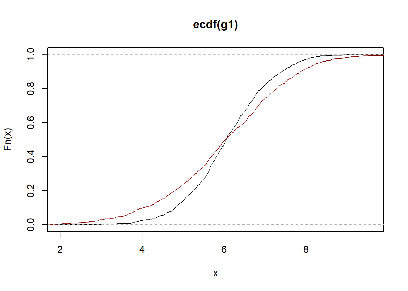
Visible here is the reason for concern: there is no meaningful change in means which is often the initial “red flag” that invites further scrutiny - but a marked change in the variance.
t.test(g1,g2)
    Welch Two Sample t-test

data:  g1 and g2
t = 0.9, df = 1759, p-value = 0.4
alternative hypothesis: true difference in means is not equal to 0
95 percent confidence interval:
 -0.0597  0.1630
sample estimates:
mean of x mean of y
     6.08      6.03
And a test:
ks.test(g1,g2)
    Asymptotic two-sample Kolmogorov-Smirnov test

data:  g1 and g2
D = 0.1, p-value = 0.00001
alternative hypothesis: two-sided
Concluding Comments
KS is a non-parametric test - which means it can be deployed across all kinds of distributions. I note that Levene’s test also non-parametric.
To sum up the main point here, in forensic analysis, if we are to scrutinize proffered data, attention should go beyond differences in the means of whatever variable we are examining. For difference in means we rely on the conventional t-test. But t-test require data that is normally, independently distributed and that the variances be equal.
But there may be data drift present - often referred to as heteroscedasticity - which vitiates the validity of the ttest. There are different methods for testing whether the variance differs between two distributions. In his Chapter 9, Nigrini does an excellent job in flagging this artifact. Both the Levene test used by Nigrini and the Kolmogov-Smirnoff (I recommend) are non-parametric - which means it applies across any data distribution you may come across.