The Computer Says No. What About It?
Computer says no. (“coughs”)
Carole Beer (Little Britain)
Contrary to popular opinion societal apprehension and the public push towards transparency in algorithmic solution for decision-making did not start with Carol Beer from Little Britain fame.
By it may have started with the uproar surrounding the Loomis decision. In Loomis, plaintiff was not allowed to examine the inner workings of a proprietary re-offender risk-assessment tool known as COMPAS.
Interrogating machine learning tools appears to have now been institutionalized by the General Data Protection Regulation (“GDPR”) in the European Union. This codifies peoples distrust of black-box algorithms and the associated “trust-me, I am the expert” culture surrounding it. This particular trend will probably be hastened along by US State data protection legislation, Connecticut being the latest of a spate of US State legislatures to launch a version on July 1st of 2023, (CTDPA).
What does this mean? Among other things, this will enhance the appeal of easier to understand algorithms and most-likely place a premium on human-in-the-loop decision-making processes.
To be sure, arguments thrusting one algo against another go back awhile. The Linear Probability Model vs. the Logit (or Probit) has been a long-standing example of the tension between clarity and statistical power (which, as it turns, out is not as straightforward (see also, Gomila, 2020 ). I have yet to see a better characterization of the issues with the Logistic than Hellevik (2009).
“… making sense of logistic regression is daunting. The technique involves unfamiliar terms such as logged odds, odds, predicted probabilities, marginal effects, log likelihood values, pseudo-variance explained, and maximum likelihood estimation that can make meaningful interpretation of results difficult.”
In fact, this LPM v Logistic comparison necessarily comes up in both Supervised Machine Learning, and Econometrics classes, ironically, the poster children of “data modeling culture” part of the statistical analysis divide (e.g. see Zhao & Hastie, 2018).
The premium on clarity and transparency in statistical modeling has long been evident to forensic economists. Its not only the trier-of-fact that needs to understand your model but counsel as well - on both sides.
The LPM v Logistic case will always be a point of contention in litigation; the one case that comes to mind is Gutierrez v. Johnson Johnson (Gutierrez v. Johnson Johnson, No. 01-5302 (WHW) (D.N.J. Nov. 6, 2006)). In Gutierrez, and with no sense of irony plaintiffs challenged defense experts’ use of the linear probability model. Gutierrez aside, it may the case that is precisely the lack of clarity that may be the source for the ensuing “battle of the experts” and “statistical dueling” and the legal strategy of using experts to neutralize opposing expert. Of course, modeling clarity is not the only route available. Other suggestions include calls for revealing the power of statistical tests proffered in testimony (e.g. Rodriguez & McGee, 2018 ) and reliance on peer-review experts to vet statistical expert reports (e.g.Hersch & Bullock, 2014 ), among others.
However, although less is more this may not be the case in the novel incantations of fraud litigation such as credit-card fraud and click-fraud. Underscoring security measures against these threats have resulted in highly complex machine learning algorithms. See for instance the solutions posted in the leaderboards of the following Kaggle fraud competitions: see here for fraudulent transactions, and here for click fraud .
At any rate, this post is to convey a sense of the debate and perhaps more importantly, to illustrate the use of the tools available to bridge this divide both for analytics and for forensics. I will use the Logistic Classification model as a stand-in for the classification “dark boxes” out there. My argument it that the difficulties with the Logistic are sufficiently onerous that most of use - analysts, instructors, economic experts - will seek easier-to-understand-and-explain models, ideally without losing predictive accuracy. The obvious alternative to the Logistic that comes to mind is the Linear Probability Model (“LPM”). But there are also others that are quite amenable for classification analysis. The One Rule (OneR) algorithm and the Fast and Frugal Trees (FFT) algorithm are quite impressive alternatives.
The Model
The objective here is to provide a refresher on choices available to analysts at the simplicity end of the spectrum.
The Data
I use the business failure data from O’Haver (1993) who used it to illustrate the use of Multiple Discriminant Analyais in commercial litigation.1
There are several benefits to using this data set. It was drawn from extant litigation. In litigation we typically do not have the luxury of large data sets nor do we often get to choose desired variables ahead of time.
Importantly, O’Haver outlined several uses for the method that are still applicable.
Analyzing a “failing firm” defense on behalf of an acquirer in a horizontal merger or acquisition. If it can be demonstrated that the target firm is likely to fail absent the acquisition, then the likelihood for regulatory or judicial approval of the merger is enhanced.
Determining whether there is justification, on the basis of financial grounds, for the termination of a poorly performing distributor or franchisee in a dealer termination litigation.
If it can be demonstrated, in certain lender liability cases, that the plaintiff firm’s financial performance has deteriorated to a point where failure is likely, justification may be provided on behalf of the lending institution in limiting future funds.
In a class action securities litigation, it may be important to demonstrate that the cause of a firm’s failure was unrelated to actions of the defendant. That is, if it can be demonstrated that independent market forces (such a drop in demand due to recession coupled with the firm’s leverage characteristics) - and not the actions of a defendant - led to financial failure, then the defendant’s liability arguments may become more supportable.
Outcome Variable
- Group Status: whether a firm had Failed or remained Viable
Predictor Variables
Inventory Turnover
Profit Margin on Sales
Return on Equity
Debt to Equity
Average Collection Period
Outcomes
suppressWarnings({
ohaver = read.csv("ohaver.csv",
                  header = TRUE,
                  stringsAsFactors = TRUE)

table(ohaver$GroupStatus)

})
FAILED VIABLE
    10     23
Results
The issue here is that the Loan Approval variable is a categorical one documenting whether a loan applicant was approved or not. And the task is to utilize other variables to develop a model to predict the likelihood of another customer getting a loan approved.
To avoid overfitting we first fit the models on a subset of the data and assess its performance on a second, “out of sample” data. The metric that we use to compare performance is Accuracy. Accuracy is the proportion of correct predictions to the total number of predictions.
A little caveat regarding accuracy. In some instances, the categorical variable we are interested in may be lopsided, that is to say many more of one category than the other. If we were examining instances of click-fraud in customer transactions, for example, clicks identified as fraudulent may be a fraction of the total data assembled. Common sense calls for adjusting the data set to “balance” it.
ohaver$GroupStatus = as.numeric(ohaver$GroupStatus) - 1
ohaver = ohaver %>% dplyr::mutate(id = row_number())
  set.seed(12345)
ohaver_train = ohaver %>% sample_frac(.70)
ohaver_test = anti_join(ohaver, ohaver_train, by = 'id')
The Linear Probability Model
The linear probability model relies on linear regression for fit.
Confusion matrix for LPM
suppressWarnings({

    model_lp <- lm(GroupStatus ~
                   InventoryTurnover +
                   PretaxROS +
                   ROE +
                   DebtToEquity +
                   COLLPD,
                data=ohaver_train)

 pred_lp = predict(model_lp, ohaver_test)

    pred_lp_qual = ifelse(pred_lp >= 0.5, 1, 0)

    tab_lp = table(pred_lp_qual, ohaver_test$GroupStatus)

colnames(tab_lp) = c("Failed", "Viable" )
colnames(tab_lp) = paste0("Approve:",colnames(tab_lp), sep = "")

rownames(tab_lp) = c("Failed", "Viable" )
rownames(tab_lp) = paste0("Predict:",rownames(tab_lp), sep = "")

tab_lp

})
pred_lp_qual     Approve:Failed Approve:Viable
  Predict:Failed              2              1
  Predict:Viable              1              6
Accuracy
lpm_result = paste0("LPM accuracy = ",round(mean(as.numeric(pred_lp_qual) == ohaver_test$GroupStatus),3) , sep = " ")

lpm_result
[1] "LPM accuracy = 0.8 "Logistic Regression
    model_glm <- glm(GroupStatus ~
                   InventoryTurnover +
                   PretaxROS +
                   ROE +
                   DebtToEquity +
                   COLLPD,
                   family =  "binomial",
                data=ohaver_train)


model_glm_pred = predict(model_glm, ohaver_test)
model_glm_pred_qual = ifelse(model_glm_pred >= 0.5, 1, 0)

tab_logit =     table(model_glm_pred_qual, ohaver_test$GroupStatus)


colnames(tab_logit) = c("Failed", "Viable" )
colnames(tab_logit) = paste0("Actual:",colnames(tab_logit), sep = "")

rownames(tab_logit) = c("Failed", "viable" )
rownames(tab_logit) = paste0("Predicted:",rownames(tab_logit), sep = "")

tab_logit
model_glm_pred_qual Actual:Failed Actual:Viable
   Predicted:Failed             0             1
   Predicted:viable             3             6
logistic_result = paste0("Logistic accuracy = ", round(mean(model_glm_pred_qual == ohaver_test$GroupStatus),3), sep = " ")
logistic_result[1] "Logistic accuracy = 0.6 "Fast & Frugal Trees
Fast-and-frugal trees (FFTs) is a simple algorithm that facilitate efficient and accurate decisions based on limited information.
    suppressWarnings({
    ohaver_train$GroupStatus = as.logical(ohaver_train$GroupStatus)
    ohaver_test$GroupStatus = as.logical(ohaver_test$GroupStatus)

    loanapp.fft = FFTrees(formula =
                           GroupStatus ~
                   InventoryTurnover +
                   PretaxROS +
                   ROE +
                   DebtToEquity +
                   COLLPD,
                         data=ohaver_train,
                         data.test = ohaver_test,
                         main = "Action",
                         quiet = TRUE,
                         decision.labels = c("Viable", "Do Not Failed")
    )


predict_fft = predict(loanapp.fft, newdata = ohaver_test)

tab_fft = table(predict_fft, ohaver_test$GroupStatus)

colnames(tab_fft) = c("Failed", "Viable" )

colnames(tab_fft) = paste0("Actual:",colnames(tab_fft), sep = "")
rownames(tab_fft) = c("Failed", "Viable" )

rownames(tab_fft) = paste0("Predicted:",rownames(tab_fft), sep = "")

tab_fft
    })
predict_fft        Actual:Failed Actual:Viable
  Predicted:Failed             1             1
  Predicted:Viable             2             6
FFT_result = paste0("FFT accuracy = ", round(mean(predict_fft == ohaver_test$GroupStatus),3), sep = " ")
FFT_result[1] "FFT accuracy = 0.7 "Plot an FFT applied to test data:
plot(loanapp.fft) 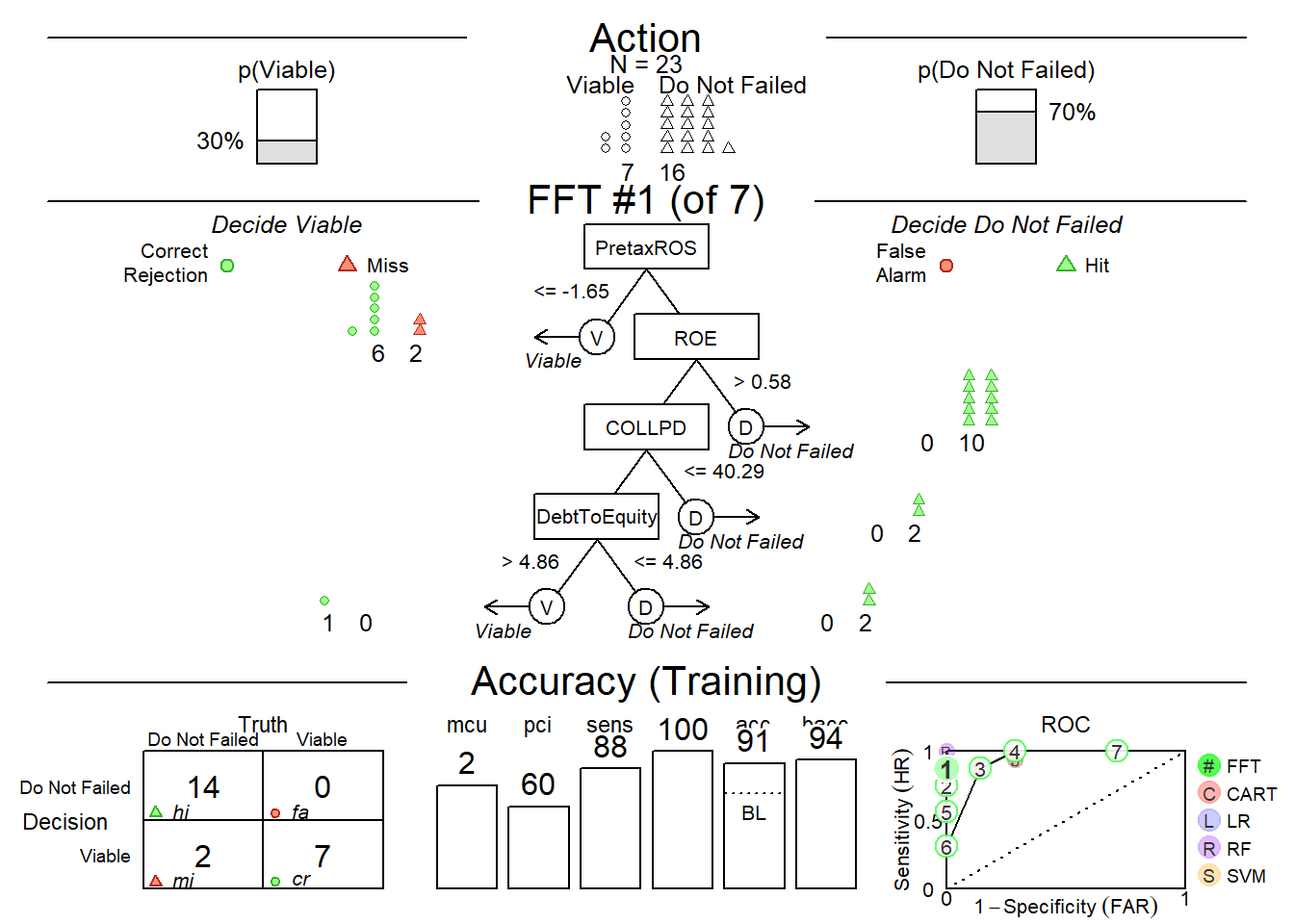
OneR with Binning
The “One Rule” algorithm generates one rule for each feature in the data and selects the rule with the smallest total error as its “one rule”.
ohaver$GroupStatus = as.factor(ohaver$GroupStatus)
data_opt = optbin(ohaver[,1:6])
data_opt %<>% dplyr::mutate(id = row_number())
  set.seed(12345)
data_opt_train = data_opt %>% sample_frac(.70)
data_opt_test = anti_join(data_opt, data_opt_train, by = 'id')

    data_opt2 <- optbin(formula =
                      GroupStatus ~
                   InventoryTurnover +
                   PretaxROS +
                   ROE +
                   DebtToEquity +
                   COLLPD,
         data=data_opt_train)

    model_opt2 = OneR(data_opt2, verbose = TRUE)
    Attribute         Accuracy
1 * PretaxROS         78.26%
1   COLLPD            78.26%
3   InventoryTurnover 73.91%
4   ROE               69.57%
4   DebtToEquity      69.57%
---
Chosen attribute due to accuracy
and ties method (if applicable): '*'
pred2 = predict(model_opt2, data_opt_test)OneR_Bin_result = paste0("One Rule with Binning accuracy = ", round(mean(as.numeric(pred2) == as.numeric(data_opt_test$GroupStatus)),3), sep = " ")
OneR_Bin_result[1] "One Rule with Binning accuracy = 0.7 "lpm_result[1] "LPM accuracy = 0.8 "logistic_result[1] "Logistic accuracy = 0.6 "FFT_result[1] "FFT accuracy = 0.7 "OneR_Bin_result[1] "One Rule with Binning accuracy = 0.7 "And the winner is … not the logistic.
As is always the case, these algorithms are susceptible to the amount and quality of the data.
Footnotes
Robert R. O’Haver, “Using Multiple Discriminant Analysis in Business Litigation”, Journal of Forensic Economics, Vol 6, No. 2 (1993), pp: 153-158↩︎