Is There an Obligation to Scrutinize Data?
Most Expert Reports prepared by Forensic Experts contain some version of the following statement:
Documents used in this report were provided to us by counsel. We conducted no independent audit or assessment of the veracity or soundness of any of the documents provided to us on this matter.
This applies practically to all documents produced in a course of an engagement - including the data underscoring our expert report and analysis - assuming of course, that we are not being asked to examine allegedly fraudulent data.
As for everything else, we are unlikely to think that documents exchanged in legal proceedings could be altered or deliberately manipulated. I suppose we take solace in our understanding of the ethical implications and the severity of the legal repercussions of submitting false documents or altering documents. And moreover, we are presumably immunized from any liability from any chicanery or deliberate misrepresentation by our client.
But should we scrutinize the data more closely?
Establishing the premise is not easy. Data could be just the wrong one - an honest mistake. It could be a result of behavioral peccadilloes. It could be someone’s innocent penchant for rounding. Or it could be that the data is made up.
The methods discussed here assist in identifying whether data is probably funky, but do not distinguish among the plausible or possible “reasons.”
Scrutinizing the Data
If we choose to examine the data, there are a number of readily available tools across various open source packages, especially in R.
We can rely on what is known as Digit Preference Analysis, and relatedly, Number-Bunching. We would use Digit Preference to examine whether the positions of a number present in a any particular data point occurs with a greater frequency that is expected. And we would use Number-Bunching to analyze the frequency with which values get repeated in the data set.1
Expected in what way? Benford’s Law is the foundation underscoring Digit Preference analysis - a practice routinely used by auditors and fraud analysts. Benford’s law (Benford, 1938) describes a pattern in many naturally-occurring numbers.2 According to Benford’s law, each possible leading digit d in a naturally occurring set of numbers occurs with a probability p(d)
\[ probability(digits) = log_{10}(1 + /digit) \]
for digits from 1 to 9.
digits =  1:9

p_d <- log10(1 + (1/digits))

stargazer::stargazer(cbind(digits,Prob_of_Occurrence = p_d),type = 'text')
=========================
digits Prob_of_Occurrence
-------------------------
1            0.300
2            0.200
3            0.100
4            0.100
5            0.080
6            0.070
7            0.060
8            0.050
9            0.050
-------------------------
Thus, with Benford’s distribution of digits as the benchline, the distribution of leading digits in data proffered in litigation can be extracted and tested against the expected frequencies.
Benford’s logic indicates that a presumption of “funkiness” is raised if the test or tests are contrary to expected results - presumably using a statistical significance threshold - although Nigrini offers a more nuanced alternative criteria.
There are various R packages available for this analysis. I list the ones I know here, in reverse order of publication.
BeyondBenford: Compare the Goodness of Fit of Benford’s and Blondeau Da Silva’s Digit Distribution to a Dataset
benford.analysis: Benford Analysis for Data Validation and Forensic Analytics
BenfordTests: Statistical Test for Evaluating Conformity to Benford’s Law
To illustrate the Benfordian methods we use the Employee Data set used by Schaefer and Visser (2003).3 This data set originates with SPSS and is referred to by Schaefer and Visser as “a standard employee data,” which suggests that it is a toy set rather than real data. In fact, given our conclusions below - which finds any number of violations between our data and the benchlines set forth - we suspect that it is a toy set.
The Employee Data set has the following variables and characteristics:
N = 474
Gender: Male/Female employee, coded Male = 1
Educ: Educational level, years
JobCat: Employment Category
1 = Clerical
2 = Custodial
3 = Managerial
Salary: Current Salary, dollars
SalBegin: Beginning Salary, dollars
JobTime: Months since hire
PrevExp: Previous Work Experience, months
Minority: Minority Status, coded 1 = minority
stargazer::stargazer(EmpData[,c(2,4:10)], type = 'text')
==================================================
Statistic  N     Mean     St. Dev.   Min     Max
--------------------------------------------------
educ      474   13.000     3.000      8      21
jobcat    474   1.000      0.800      1       3
salary    474 34,420.000 17,076.000 15,750 135,000
salbegin  474 17,016.000 7,871.000  9,000  79,980
jobtime   474   81.000     10.000     63     98
prevexp   474   96.000    105.000     0      476
minority  474   0.200      0.400      0       1
--------------------------------------------------Hmisc::hist.data.frame(EmpData[,c(2,4:5)])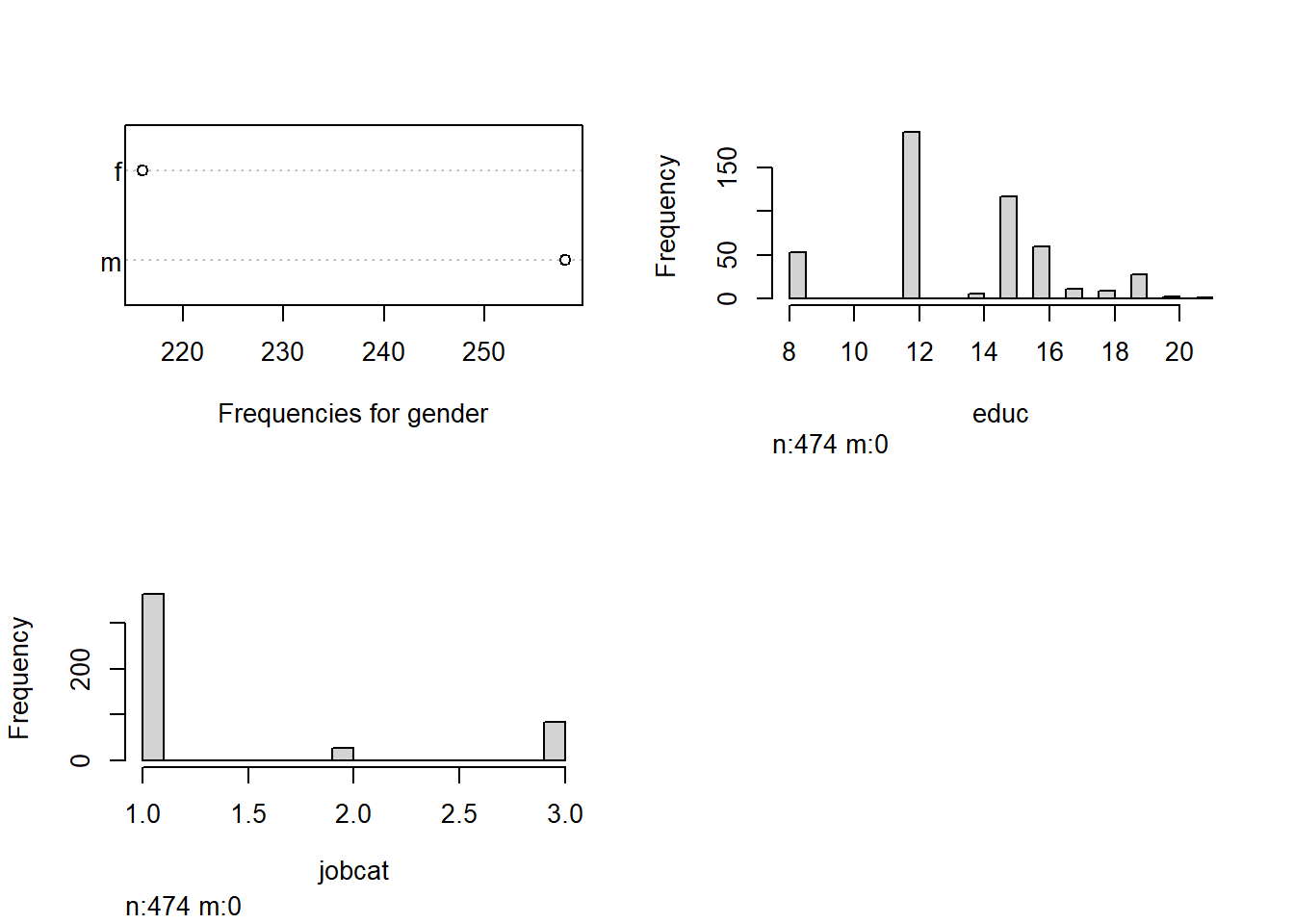
hist(EmpData[,c(6:10)])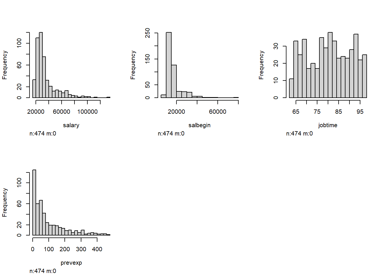
The Distribution of Digits
Here we extract the first digits of the entire salary series.
first_digits = substr(format(EmpData$salary,
                              trim=TRUE),1,1)
digit1 = table(factor(first_digits,levels=paste(digits)))
digit1
  1   2   3   4   5   6   7   8   9
38 225 112 32 25 22 11 5 4 prop.table(digit1)
    1     2     3     4     5     6     7     8     9
0.080 0.475 0.236 0.068 0.053 0.046 0.023 0.011 0.008 barplot(digit1, xlab = "digits", ylab = "counts",
main = "Employee Data Set")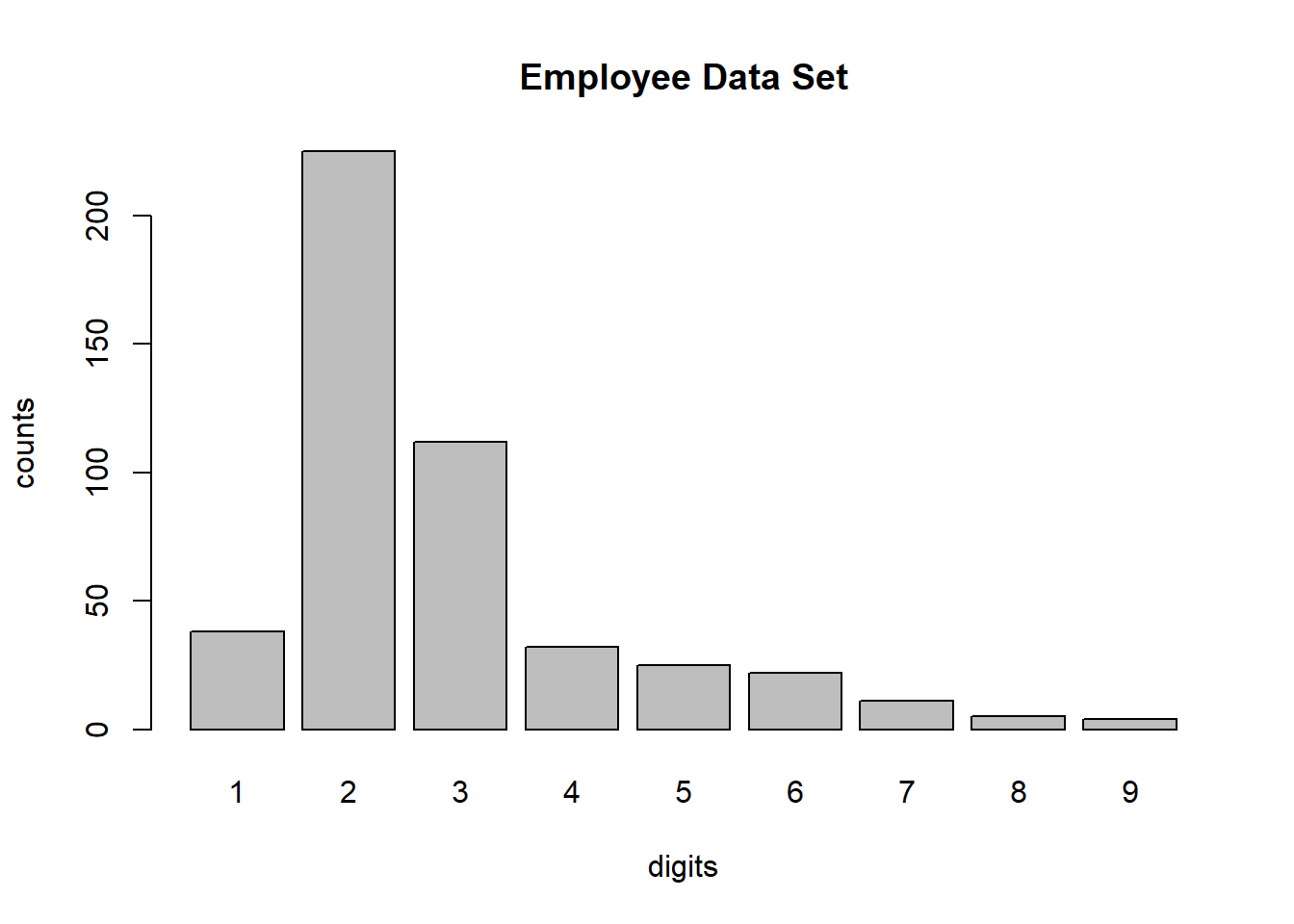
Here is the first step, testing the compatibility of the leading digit to the Benford expected count benchline.
x = digit_test(EmpData$salary, check = "first", reference = "benford")
    x
    Digit distribution test

data:  EmpData$salary
n = 474, X-squared = 521, df = 8, p-value <0.0000000000000002
alternative hypothesis: leading digit(s) are not distributed according to the benford distribution.
The results are pretty clear: the series do not match. Here is a visual depiction of both series.
plot(x)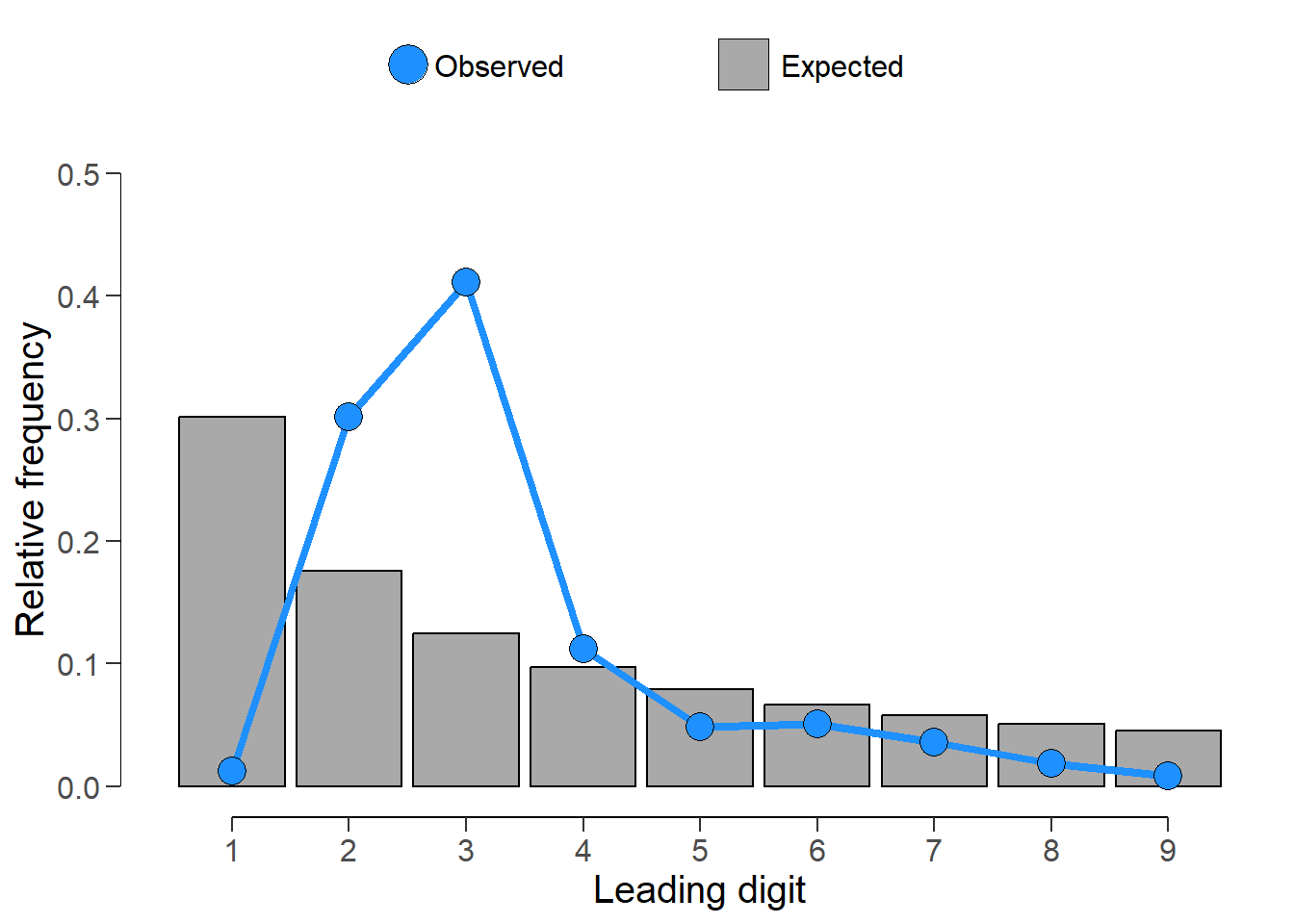
It turns out that Benford’s law extends not only to the first digit but also to the others:
\[ p(D_{1}=d_{1}, D_{k}=d_{k}) = log_{10}(1 + 1/\sum_{i = 0}^k(10^{k-i}d_{i})) \]
for all: \(d_{1} \; \in \; \{1,...,9\}\), and
all other: \(d_{j} \; \in \; \{0,...,9\}, j = 2,...,k\).
xx <- digit_test(EmpData$salary, check = "firsttwo", reference = "benford")
xx
    Digit distribution test

data:  EmpData$salary
n = 474, X-squared = 8187, df = 89, p-value <0.0000000000000002
alternative hypothesis: first two digit(s) are not distributed according to the benford distribution.
Display of the expected frequency versus actual frequency for the first two digits of the salary series.
plot(xx)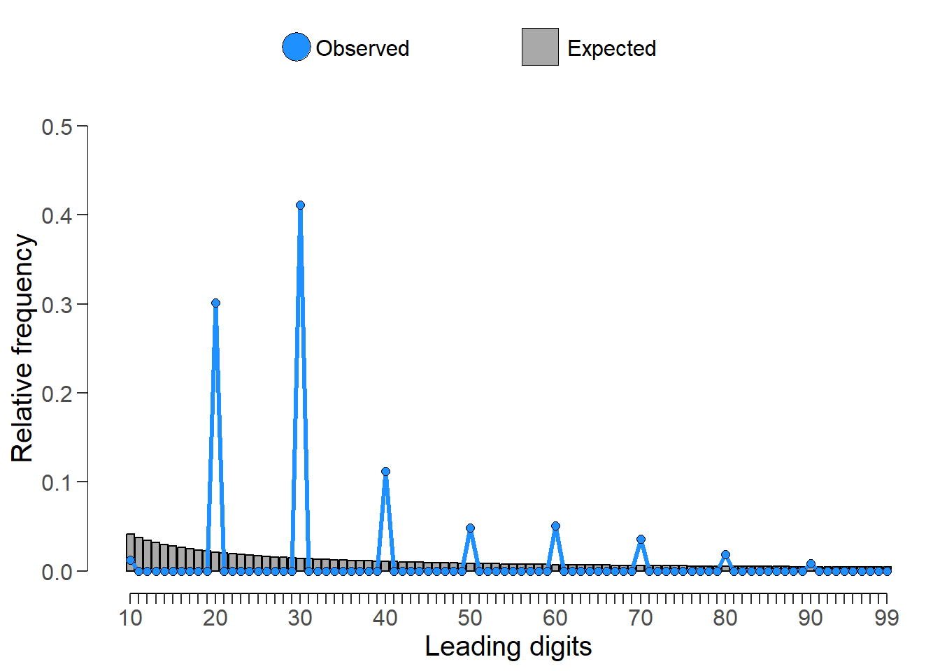
Both tests are rejected conclusively, and as such suggest that the salary data does not conform to Benford’s Law.
The mean absolute deviation or mean square error is a popular statistic commonly used in forensic analysis. It is a the average of the squared differences between the actual values and the expected values. Nigrini argued that MAD more closely reflects the similarity of a data series to the expected Benford series - and thus, recommended MAD over p-values. The gauge is known as MAD conformity (to Benson’s Law).4
The R package benford.analysis provides estimates of MAD and specifically establishes whether MAD conforms to Benford. Interestingly, it warns perhaps judiciously, to avoid exclusive reliance on the p-statistic for decisionmaking.
      bfd.mdf = benford(EmpData$salary)
      plot(bfd.mdf)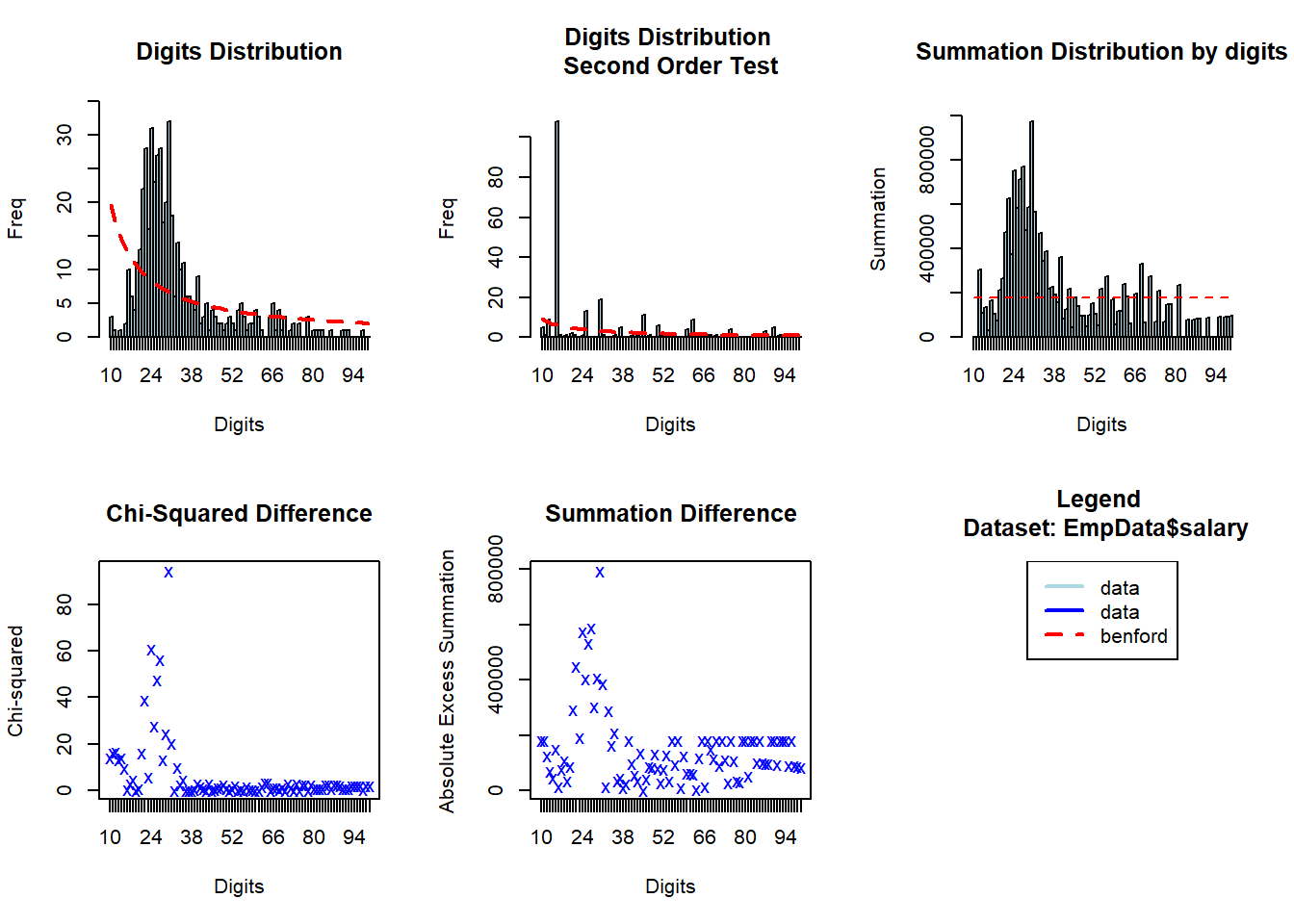
Among the results displayed above is the one for a “summation test” testing against the “summation distribution.”5 The summation test scrutinizes for excessively large numbers in the data series. It identifies numbers that are larger than the norm for the series. The sums of all numbers in a Benford distribution with first two-digits should be the same. Accordingly, each of the 90 first-two digits groups sum proportions should be equal, that is to say, 1/90 or 0.011. Spikes or bunching visible in the plot indicate that there are some large single numbers or set of numbers.
bfd.mdf
Benford object:

Data: EmpData$salary
Number of observations used = 474
Number of obs. for second order = 220
First digits analysed = 2

Mantissa:

   Statistic Value
        Mean 0.487
         Var 0.029
 Ex.Kurtosis 0.494
    Skewness 0.670


The 5 largest deviations:

  digits absolute.diff
1     30            25
2     24            23
3     27            21
4     26            19
5     22            19

Stats:

    Pearson's Chi-squared test

data:  EmpData$salary
X-squared = 597, df = 89, p-value <0.0000000000000002


    Mantissa Arc Test

data:  EmpData$salary
L2 = 0.4, df = 2, p-value <0.0000000000000002

Mean Absolute Deviation (MAD): 0.01
MAD Conformity - Nigrini (2012): Nonconformity
Distortion Factor: -15

Remember: Real data will never conform perfectly to Benford's Law. You should not focus on p-values!
We can identify the “suspicious” observations in the data set. Presumably, in this context, the salaries that do not conform to Benford. And, surprisingly, none of the suspicious ones appear to be within the managerial ranks.
suspects = getSuspects(bfd.mdf, EmpData)
suspects %>% group_by(jobcat) %>% count()
# A tibble: 2 × 2
# Groups: jobcat [2]
jobcat n
<int> <int>
1 1 45
2 2 18Here are those within the Custodial job category. There are 18. We show the top six.
suspects %>% filter(jobcat == 2) %>% head() id gender bdate educ jobcat salary salbegin jobtime prevexp minority
1: 45 m 1938-08-02 12 2 30750 13500 95 307 0
2: 48 m 1947-06-07 12 2 30750 14100 94 240 0
3: 96 m 1933-10-02 8 2 30750 15000 92 432 1
4: 98 m 1956-05-17 8 2 30000 15000 92 144 1
5: 111 m 1940-11-27 12 2 30750 9000 91 314 1
6: 112 m 1948-06-21 12 2 30750 15000 91 240 1Here are those within the Clerical job category. There are 45 of these.
suspects %>% filter(jobcat == 1) %>% head() id gender bdate educ jobcat salary salbegin jobtime prevexp minority
1: 10 f 1946-02-13 12 1 24000 13500 98 244 0
2: 11 f 1950-02-07 16 1 30300 16500 98 143 0
3: 23 f 1965-03-15 15 1 24000 11100 97 75 1
4: 47 f 1938-04-28 12 1 30000 16500 95 228 0
5: 60 m 1959-02-16 12 1 30900 15000 94 102 1
6: 75 f 1965-08-12 15 1 24150 11550 93 0 0Interestingly, the fact that the nonconformity avoids the managerial ranks is of itself an artifact of this data set that raises a presumption of its “funkiness,” perhaps to be further investigated. And come to think of it, this lack of managerial salary-data fudging questions my thesis that this data is synthetic.
Number Bunching
Number bunching is a procedure attributed to Uri Simohnsohn.6
The point of this analysis is to examine the frequency with which values get repeated within a set of numbers. this approach examines the entire number at once, not only the first or last digit - as in digit analysis [See, Simohnsohn (2019)].
To determine whether the data show an excessive amount of bunching, the null hypothesis that x does not contain an unexpected amount of repeated values is tested against the alternative hypothesis that x has more repeated values than expected. The statistic can either be the average frequency
\[ Average Frequency = \sum(f_i^2)/\sum(f_{i}) \]
of the data or the entropy
\[ Entropy = -\sum(p_{i}*log(p_{i}) \]
where:
\[ p_{i} = f_{i}/np_{i} = f_{i}/n \]
Average frequency and entropy are highly correlated. An average frequency of 2.5 means that, on average, your observations contain a value that appears 2.5 times in the data set.
x <- repeated_test(EmpData$salary,
                       check = "all",
                       method = "entropy",
                       samples = 2000)
Warning in cor(x, y): the standard deviation is zerox
    Repeated values test

data:  EmpData$salary
n = 474, S = 5, p-value = 1
alternative hypothesis: entropy in data is lower than for random data.
Number-bunching draws on the measure of entropy. Entropy is a concept from Information Theory with wide-ranging applications. Entropy measures the amount of information held in data; specifically, to what extent the data are “spread out” over its possible values. Thus, a variable displaying high entropy means that the data are spread out as much as possible while low entropy means that the data are “bunched-up,” or nearly all concentrated on one value.
Here is a visible display of the “bunching-up” of the salary series.
plot(x, col = "dark red", lwd = 10)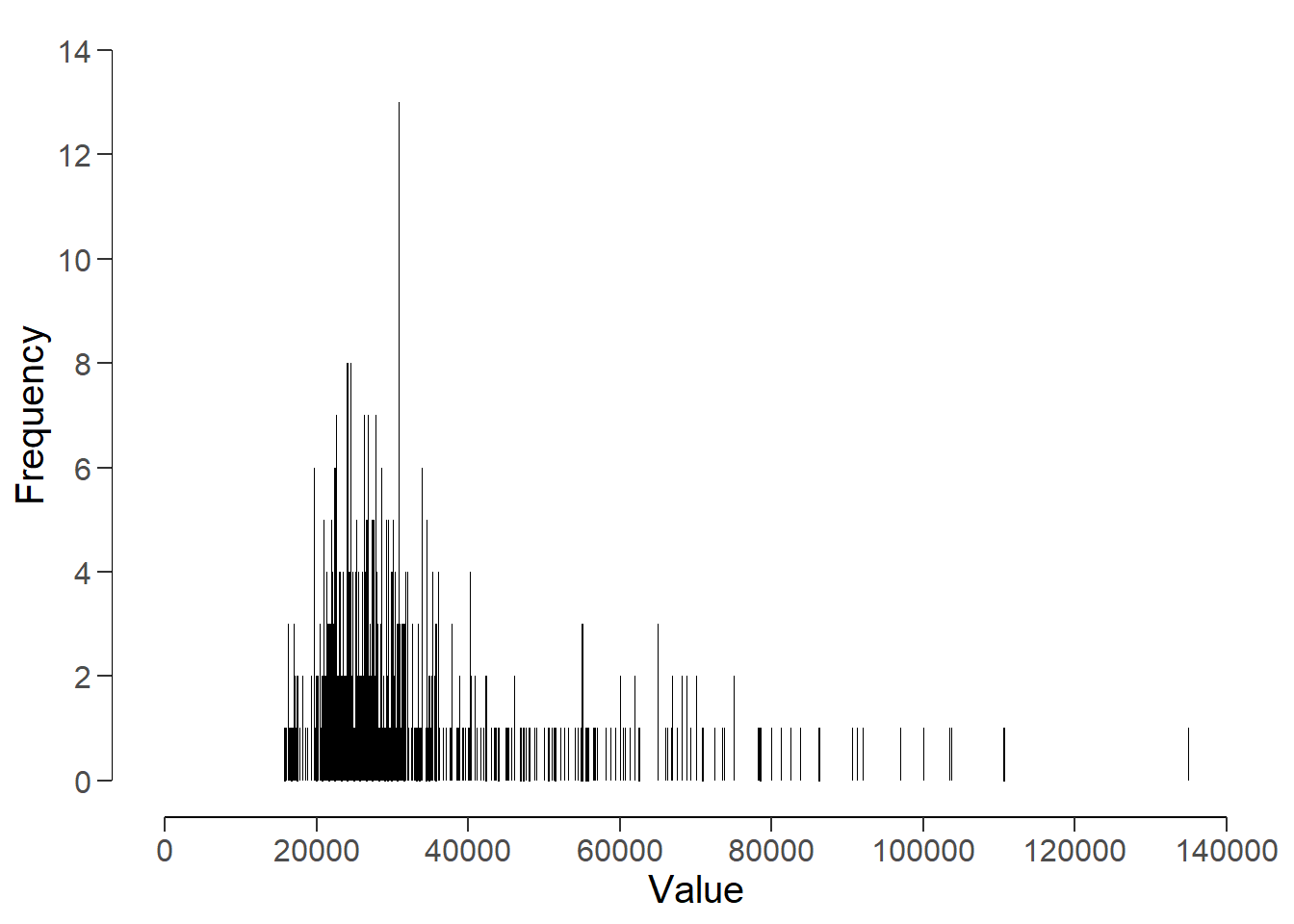
For our purposes, bunched-up data is more likely to be an artifact. To illustrate, here we show the visual representation of the salary data and a random draw of the same data.
   Min. 1st Qu.  Median    Mean 3rd Qu.    Max.
  15750   24000   28875   34420   36938  135000
[1] 6[1] 6The salary data shows less “randomness” (i.e. number-bunching) when compared to a random draw.
x3rand=as.vector(t(sample(EmpData[,6],
                      length(EmpData[,6]),
                      replace = T)))

x3=as.vector(t(EmpData[,6]))


levels_salary=seq(from=15000,to = 150000,by = 1000 )
t3=table(factor(floor(x3),levels=levels_salary))


t3rand = table(factor(x3rand,levels=levels_salary))

mydata= data.frame(levels_salary,t3, t3rand)


colnames(mydata)[c(3,5)] = c("Actual", "Random")

    g1 = ggplot(mydata,
          aes(x = levels_salary,
              y = Actual,
              col = as.factor(levels_salary))) +
        geom_col() +
        theme(legend.position = "NULL")+
        labs(x = "Salary")

  g2 = ggplot(mydata,
        aes(x = levels_salary,
        y = Random,
        col = as.factor(levels_salary))) +
        geom_col() +
        theme(legend.position = "NULL") +
        labs(x = "Salary")

  cowplot::plot_grid(g1, g2,
                     label_size = 10,
  labels = c('Employee Data, Actual',
             'Employee Data, Randomized'))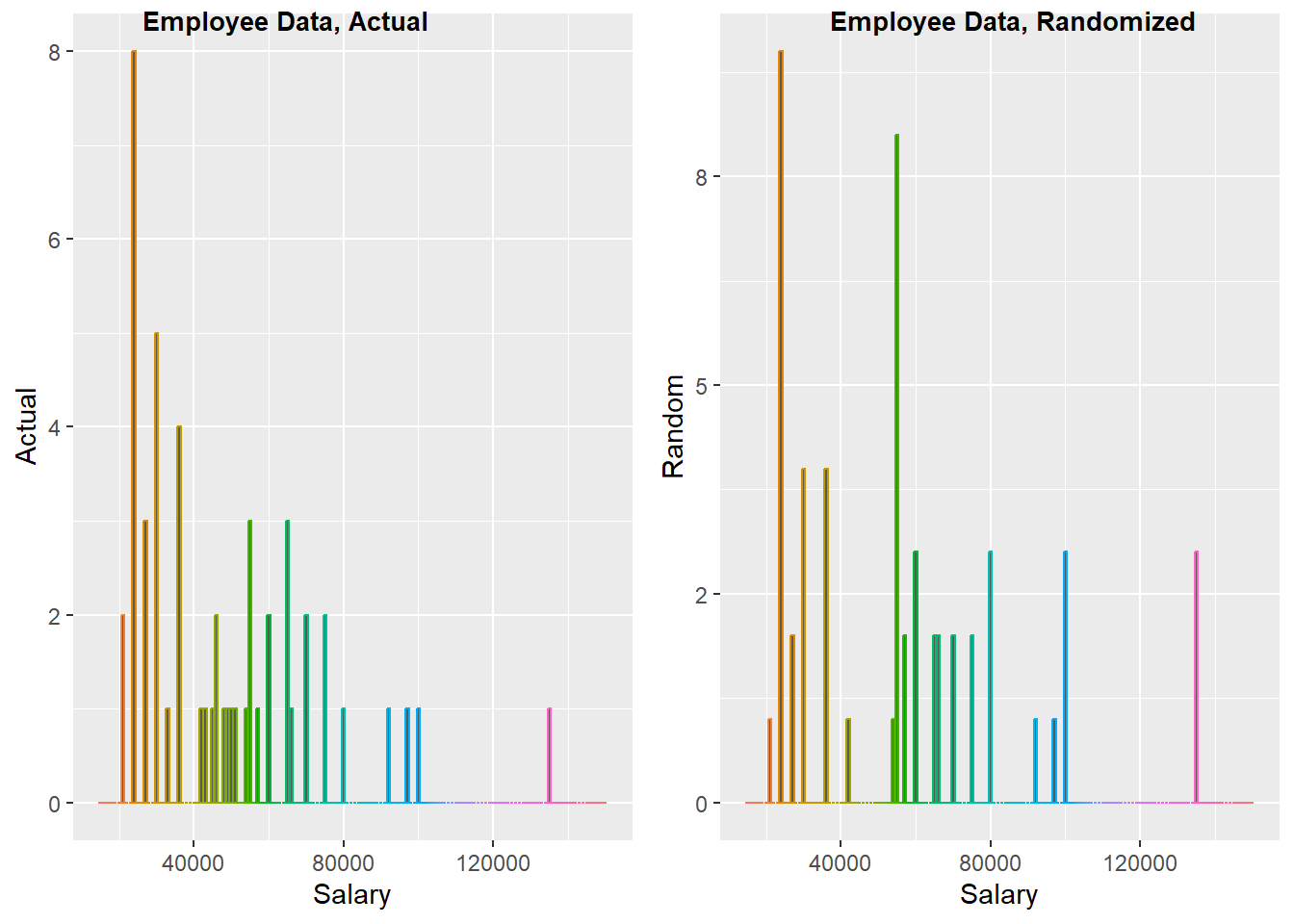
Conformity to Benford’s distribution across several dimensions cannot be confirmed for salary series of the Employee data set used by Schaeffer and Visser. To the contrary, we found considerable evidence of deviations from Benford’s Law based on examinations of the first, last and first and last digit for the salary series.
We also found notable instances of “bunching” typical of fraudulent representation, deliberate manipulations, inaccuracies or biases in proffered data. I remain partial to believing that this data is synthetic .
Footnotes
This does not refer to the technique of estimating parameters of behavioral responses that uses mass points in a a distribution. - which is also called bunching.↩︎
Benford, F., “The Law of Anamalous Numbers,” Proceedings of the American Philosophical Society (1938), pp: 551-572.↩︎
Schaefer, Kurt C., and Michelle L. Visser, “Reverse Regression and Orthogonal Regression in Employment Discrimination Analysis,” Journal of Forensic Economics, Volume 16, No. 3, (2003), pp:238-298↩︎
Nigrini, M. J., Benford’s Law: Application for Forensic Accounting, Auditing and Fraud Detection (New Jersey: Wiley and Sons, 2012).↩︎
Nigrini, M. J., Benson’s Law: Applications in Forensic Accounting, and Fraud Detection, (New Jersey, John Wiley & Sons: 2012)↩︎
Simohnsohn, Uri. Number-Bunching: A New Tools for Forensic Data Analysis, (May 25, 2019).↩︎